Exploring Word2Vec Embeddings
Let’s dive into a concept that is very important in natural language processing which is to find a representation for words that a computer can understand. Words in a computer can be represented as an array of bytes encoded as ASCII characters. This format is however not very flexible when trying to capture the meaning of a word in a corpus. Another approach is to use the one-hot encoding where each unique word has a one in the vector and zeroes everywhere else.
Vocabulary: ["hello", "world", "apple", "cat"]
Vector embeddings:
"hello": [1, 0, 0, 0]
"world": [0, 1, 0, 0]
"apple": [0, 0, 1, 0]
"cat":   [0, 0, 0, 1]
There are many problems with one-hot encoded vectors:
- The size of the vocabulary is tied to the number of dimension as the vocabulary becomes very large the vectors become extremley large, and wastes memory by needing to store mostly zeroes. The large dimensions are commonly referred to as the curse of dimensionality.
- These vectors are not capable of capturing any meaning in words since each word gets its own dimension.
- The vectors are very closely coupled to their application which means they are practically useless when you change the application and the corpus used.
To solve this we need to consider words that are close together in the corpus as similar or ralated to each other and try to the represent words using only those relations called word embeddings. In order to create these word embeddings we need to create a fake neural network task which is to try and predict given one word which words that are related to that word. So the network inputs a one-hot encoded vector e.g. "hello": [1, 0, 0, 0] and then goes to a hidden layer of that has a lower dimension e.g. 2-dimensions [0.4241, 0.5832] this will start-out being random garbage but the trick is to then use gradient decent learning to evaluate the output of the network which should be any of the neighboring words in the corpus. This forces the network to learn how to represent the word "hello" that also respects the context in which it appears in the text. This is an example of how such a network could look like:
             Input (1-hot)    Hidden (embedding)       Output (softmax classifier)
               1                                       0.9834
          =>   0           =>   0.3041           =>    0.8724
 "hello"  =>   0           =>   0.1941           =>    0.1928
               0                                       0.0042
After training we can essentially extract the hidden layer and this can be used to encode our words into more meaning ful word embeddings. There are of course multiple limitations with this approach which are that
This is an unsupervised machine learning task called word2vec and can be implemented in two ways either using Skip-gram or CBOW (continuous bag-of-words). For this experiment the skip-gram approach was choosen but they are essentially the inverse of each other. For this to work skip-grams needs to be constructed they are pairs of words that are closeley related to each other and that is determinted by their distance from each other in the corpus. The window-size determines the maximum distance (in number of words) they can appear from each other. Usually window-size = 2 works well, too large window might include words that are not related to each other. The skip-grams are created by sweeping over the text word by word, for each word make that the center word and create pairs (center word, context word) where the context words are.
Model implementation in PyTorch (NOTE: this code does not represent our final code this is only experimental code):
class Word2Vec(nn.Module):
    def __init__(self, vocab_size, embedding_size):
        super(Word2Vec, self).__init__()
        self.embedding = nn.Linear(vocab_size, embedding_size, bias=False)
        self.output = nn.Linear(embedding_size, vocab_size, bias=False)

    def forward(self, x):
        x = self.embedding(x)
        return self.output(x)
The Word2Vec model has two parameters the vocab_size is the size of our vocabulary and embeddings_size is the number of dimensions to use for our final word vectors.
Hyper parameters used:
embedding_size = 30
window_size = 2
batch_size = 64
num_epochs = 5000
learning_rate=0.001
optimizer = optim.Adam(model.parameters(), lr=learning_rate)
criterion = nn.CrossEntropyLoss()
Creating the skip-grams:
word_sequence = data.word_sequence_from_korp_dataset("../dataset/" + filename)
vocab = list(set(word_sequence))
vocab_size = len(vocab)
print("vocab_size:", vocab_size)

skip_grams = list()
for i in range(1, len(word_sequence) - 1):
    center_word = vocab.index(word_sequence[i])
    for j in range(i - window_size, i + window_size):
        if j != i and j >= 0 and j < len(word_sequence):
            context_word = vocab.index(word_sequence[j])
            skip_grams.append((center_word, context_word))
num_skip_grams = len(skip_grams)
Now training this can be done in several ways but the easiest method seams to just take a few random samples from the skip-grams.
def load_samples():
    input_batch = list()
    target_batch = list()
    indices_batch = np.random.choice(range(num_skip_grams), batch_size, replace=False)
    for i in indices_batch:
        input_batch.append(np.eye(vocab_size)[skip_grams[i][0]]) # center word
        target_batch.append(skip_grams[i][1]) # context word

    inputs = torch.Tensor(input_batch)
    targets = torch.LongTensor(target_batch)
    return inputs, targets
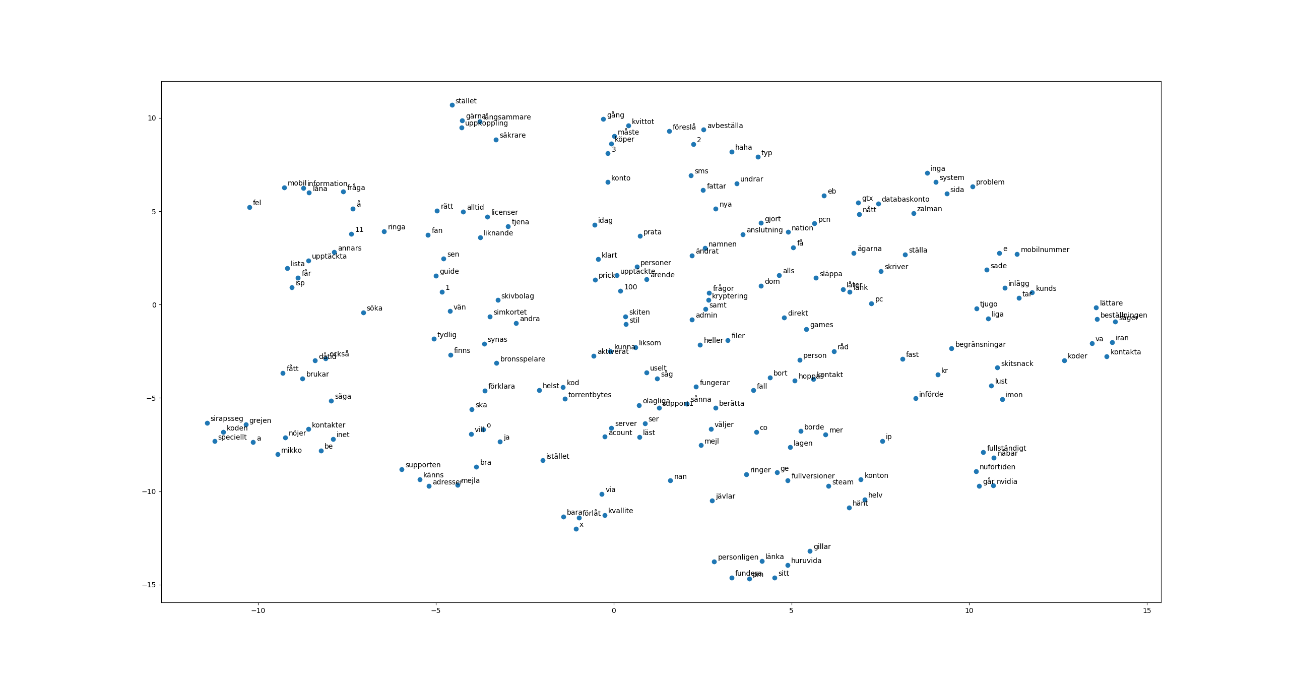
Now it is hard to properly evaluate the word embeddings but considering that the dataset was pretty small it probably wasn’t that good. Using the t-SNE dimensionality reduction technique we can get a feel for how the high dimensional word vectors are located on a scatter plot:
- References Some very helpful articles used when implementing this NLP 101: Word2Vec — Skip-gram and CBOW NLP 102: Negative Sampling and GloVe
The dataset we used for this exeriment was a subset of this Flashback: Dator och IT
/The RPA Tomorrow Team